Showing posts with label correlation. Show all posts

Monday, December 09, 2019

Added Variable Graphs

Introduction

A common difficulty in regression modeling is to figure out which input variables should be included. One tool at our disposal is the added-variable plot. Given an existing model, the added-variable plot lets us visualize the improvement we would get by adding one more variable of our choosing. This idea is described nicely in A Modern Approach to Regression with R by Simon J. Sheather, pages 162-166.

A function for displaying add-variable curves can be found in R's car package, among other places. That package is the support software for An R Companion to Applied Regression, and has other useful functions for regression modeling.

Simulated Data

To illustrate the added-variable graphs, I'll use simulated data. Simulations are useful, because when we build the relationship between variables by hand, we know what the answer is when we start. Then we can check the actual answer versus the regression model. 


library(tidyverse)
library(broom)

add_names <- function(x, .names){
  colnames(x) <- .names
  return(x)
}

# create three variables that have correlations
cm <- matrix( c( 1, .5, .6,
                 .5, 1, .3,
                 .6,.3,  1),
              nrow = 3, 
              ncol = 3)

sim_data <- MASS::mvrnorm(n = 1000, mu = c(0,0,0), Sigma = cm) %>% 
  scale() %>% 
  add_names(c("y","x","z")) %>% 
  as_tibble()

# check the variance properties
var(sim_data) %>% round(2)

    y    x    z
y 1.00 0.49 0.64
x 0.49 1.00 0.32
z 0.64 0.32 1.00

This code creates three variables: y (the output) and x,z (two inputs). They each have mean zero and variance 1, and--as you can see from the covariance matrix at the bottom--are each correlated with each other. Because of the scaling, the correlation coefficients between variables are the same as the covariances, so cor(x,y) = .49 in the sample data. Ideally it's .5, from the specification, but there's a bit of sampling error.

A Combined Model

One problem that bedevils regression analysis is that inputs can be correlated with each other, so the explanatory power of each in isolation may be quite good, but when we put them together in the model, they essentially provide the same information about the output--so the coefficients look weird. The coefficient may even have the "wrong" sign. This is not mistake; the output will always minimize squared error. Rather it's a consequence of the correlational structure of the inputs that confounds our intuition. 


m_xyz <- lm(y ~ x + z, sim_data)
summary(m_xyz)

Coefficients:
             Estimate Std. Error t value Pr(>|t|)    
(Intercept) 6.226e-17  2.250e-02    0.00        1    
x           3.145e-01  2.377e-02   13.23   <2e-16 ***
z           5.362e-01  2.377e-02   22.56   <2e-16 ***
---
Signif. codes:  0 ‘***’ 0.001 ‘**’ 0.01 ‘*’ 0.05 ‘.’ 0.1 ‘ ’ 1

Residual standard error: 0.7115 on 997 degrees of freedom
Multiple R-squared:  0.4948, Adjusted R-squared:  0.4938 
F-statistic: 488.3 on 2 and 997 DF,  p-value: < 2.2e-16

Because the means are all zero, the intercept is zero. The coefficient estimates are given by the formula \( \beta = r_{xy} s_x / s_y \) for simple two-variable models (e.g. y predicted by x alone), so in our case the individual betas would be cor(sim_data$x, sim_data$y) * sd(sim_data$y) / sd(sim_data$x) = .488. But it's less than that here, because we've added z as an explanatory variable, which is correlated with x.

Added-Variable Plots

With the two-input model, we can now ask for add-variable plots from the car package with 

car::avPlots(m_xyz)


The graph on the left starts with the model y ~ z and then figures out what the addition of x to this would add, to create y ~ x + z. The graph on the right does this in reverse, starting with y ~z and adding z. The slopes of the lines are the same as the regression coefficient that will result in the combined model for the given variable. So we want to see non-zero slopes. In this case, we can see that both of these inputs (x and z) are useful in explaining y. 

Model Outputs

Since we are comparing several models, I'll show the summary results using the broom package.


# Models
m_xy <- lm(y ~ x, sim_data)
m_xz <- lm(z ~ x, sim_data)
m_zy <- lm(y ~ z, sim_data)
m_xyz <- lm(y ~ x + z, sim_data)

# Assemble summary statistics
m_stats <- map_df(list(m_xy,m_xz,m_zy,m_xyz),glance)
m_stats$Model <- c("m_xy","m_xz","m_zy","m_xyz")
m_stats$r <- sqrt(m_stats$r.squared)
m_stats %>% select(Model,r, r.squared)
The magic happens in line 8, using the broom package's glance function to generate summary model statistics and the purrr package's map function to put them all into a data frame.


  Model     r r.squared
  <chr> <dbl>     <dbl>
1 m_xy  0.487     0.237
2 m_xz  0.321     0.103
3 m_zy  0.637     0.406
4 m_xyz 0.703     0.495

I added the r column, which is the correlation between variables. You can check the covariance matrix above and verify that these are the same values found there (e.g. m_xy predicts y from x, and has r = .487, which corresponds to the second element of the first row of the covariance matrix (rounded to .49).

Discussion

There's a lot more to say about these graphs. The mathematical motivation is found in Sheather's book. In the next article I'll unpack the geometry behind the graphs and show why they still don't entirely solve our problem with co-linearity among predictors. Still, added-value graphs are a nice tool to have in the kit.

Monday, May 26, 2014

2014 AIR Forum: Correlation, Prediction, and Causation

I've put my slides for my AIR presentation on dropbox. You can access them here. The text of my remarks is included as comments under the slides.

Friday, December 16, 2011

Free Hypothesis-Generating Software

In the last year there have been announcements of two free software packages that use machine learning techniques to mine data for relationships. The resulting mathematical formulas can be used to form hypotheses about the underlying phenomena (i.e. whatever the data represents).

The first one I have mentioned before. It's Eureqa from Cornell, which uses symbolic regression. There is an example on the Eureqa site that poses this sample problem:
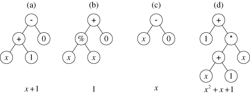
This page describes an illustrative run of genetic programming in which the goal is to automatically create a computer program whose output is equal to the values of the quadratic polynomial x2+x+1 in the range from –1 to +1. That is, the goal is to automatically create a computer program that matches certain numerical data. This process is sometimes called system identification or symbolic regression.
The program proceeds as an evolutionary search. The graph pictured below is a schematic of the way the topology of the evolved "critters" is formed.
A family tree of mathematical functions. (Image Source: geneticprogramming.com)
There is a limitation to genetic programming that is also a threat to any intelligent endeavor: the problem may not be amenable to evolutionary strategies. There are some problems where the only way to solve them is exhaustive search. Only if the solution space is "smooth" in the sense that good solutions are "near" almost-good solutions is the genetic approach going to find solutions faster than exhaustive search. On a philosophical note, modern successes with physical sciences suggest that the universe is kind to us in this regard. The "unreasonable effectiveness" of mathematics (the title of an article by Eugene Wigner) in producing formulas that model real world physics is a hopeful sign that we may be able to decode the external environment so that we can predict it before it kills us. (The internal organization of complex systems is another matter, and there's not much success to look to there.). Note, however, that even here formulas have not really been evolutionary, but revolutionary. The formulation of Newton's laws of motion are derivable from Einstein's relativity, but not vice versa. The "minor tweak" approach doesn't work very often, Einstein's Cosmological Constant notwithstanding.

The second data miner is aptly called MINE, and comes from the Broad Institute of Harvard and MIT. You can read about it on their site broadinstitute.org. The actual program is hosted at exploredata.net, where you can download a java implementation with an R interface. Here's a description from the site:
One way of beginning to explore a many-dimensional dataset is to calculate some measure of dependence for each pair of variables, rank the pairs by their scores, and examine the top-scoring pairs. For this strategy to work, the statistic used to measure dependence should have the following two heuristic properties. 
Generality: with sufficient sample size the statistic should capture a wide range of interesting associations, not limited to specific function types (such as linear, exponential, or periodic), or even to all functional relationships. 
Equitability: the statistic should give similar scores to equally noisy relationships of different types. For instance, a linear relationship with an R2 of 0.80 should receive approximately the same score as a sinusoidal relationship with an R2 of 0.80.
It's interesting that this is a generalized approach to my correlation mapper software, the difference being that I have only considered linear relationships. For survey data, it's probably not useful to look beyond linear relationships, but I look forward to trying the package out to see what pops up. It looks easy to install and run, and I can plug it into my Perl script to automatically produce output that complements my existing methods. A project for Christmas break, which is coming up fast.

Update: I came across an article at RealClimate.org that illustrates the danger of models without explanations. Providing a correlation between items, or a more sophisticated pattern based on Fourier analysis or the like, isn't a substitute for a credible explanatory mechanism. Take a look at the article and comments for more.

By coincidence, I am reading Emanaul Derman's book Models.Behaving.Badly: Why Confusing Illusion with Reality Can Lead to Disaster, on Wall Street and in Life. It has technical parts, which I find quite interesting, and more philosophical parts that leave me scratching my head. The last chapter, which I haven't read yet, advertises "How to cope with the inadequacies of models, via ethics and pragmatism." Stay tuned...

Update 2: You can read technical information about MINE in this article and supplementary material.

Friday, December 09, 2011

X-Raying Survey Data

I continue to develop and use the software I patched together to look at correlates (or covariates) within large scalar or ordinal data sets like surveys. I have gotten requests from several institutions in and out of higher ed to do these. A couple of interesting graphs that resulted are shown below, with permission of the owners of the data, who shall remain anonymous. Both of these are HERI surveys. I have found the HERI surveys the most revealing, partly because they discriminate so well between different dimensions. Some other surveys seem to produce (in the data sets I've seen) big globs of correlated items that are hard to get meaning from.

First the CIRP Freshman Survey at a private college. It neatly divides up the survey respondents into clusters. Rich urban kids negatively correlated to working class or middle class kids, athletes, the religious, and the environmentally-conscious all show up clearly. I've labeled the optional questions with an approximation of the prompt.[Download full-sized graph]
Next is the Your First Year College Survey at a different private college. I find the link between texting in class and recommending the school to others particularly interesting. That's at the bottom. Red lines are negative correlations.[Download full-sized graph]

Tuesday, October 18, 2011

Mapping covariates, Part III

In my spare time (ha-ha) I refined the software I blogged about in the last two posts in order to automate almost everything about sorting out what's connected to what in a data set.  Now I can create a folder with a data file, an index of variables, and an options list, drop that folder on a script on the desktop, and a few seconds later have a graph like the one below. This makes it easy to tweak parameters to find a nice picture. One that tells $2^{10}$ words, give or take.

For the graph below, I dug out the results of a semester of course evaluation using the new form I got implemented a year ago. I wrote previously about the odd fact that the summative evaluation of the course in Q12 and Q13 didn't seem to relate much to the learning outcomes. The closest other item in this topology is how enjoyable the students reported the course being.

This graph shows covariances instead of correlations. The latter have the nice property of being normalized to [-1,1], but suffer from the fact that nearly constant items all correlate highly with each other. The program can run either way. The graph below shows the top 30 correlates. The means are shown too.


Saturday, October 01, 2011

Creating Graphs with Perl and GraphViz

Yesterday I solved one of my data problems, but that just led to another one. I can now filter large correlation tables for (absolute) values above a threshold, but it's still laborious to connect those in a diagram that shows the relationships. So the next step was to look for a program to display graphs. Here, I don't mean bar graphs and pie charts and whatnot, but the mathematical object that was unfortunately also called a graph, which consists of vertices and edges. Or dots and lines connecting them, if you prefer. A map of a subway system is a kind of graph. Here's a very simple one:

With the correlations, I want to see what belongs with what on a graph that is generated automatically from a threshold I assign. In the example above, survey results show a perception that creativity is associated with artistic ability.

Fortunately, other people have already solved this problem, and it's just a matter of putting the machinery in place. I used two pieces of software, GraphViz (thanks to AT&T and the development team) and the perl interface for it (thanks to developer Leon Brocard). Both of these are open source and free to use.

The only other thing I had to do was extract the prompts for each item to correspond to the item codes. Otherwise, you get a nice graph showing that RATE1 connects to RATE2, which doesn't help understand what's going on.

I used the CIRP data with a .5 threshold to get these interesting networks of association. It takes just a few seconds to select the threshold value, run the scripts, and look at the resulting file. The code for generating the graphs from the output of the correlation summaries is here. There are many, many options for displaying the graphs. The gallery of GraphViz images shows off the versatility of the software.


This software does a great job of placing nodes logically so that the edges (the lines) are organized and neat.
Update: Here is a complete output with some cool new modifications.

Friday, September 30, 2011

A Recipe for Finding Correlates in Large Data Sets

The internet has revolutionized intelligence. I've seen articles about how it's making us dumber, and I don't know if that's true, but it's certainly made me spoiled. In the old days if I had a computer problem I would just use brute trial and error, often giving up before finding a solution. Now, I just assume that someone else has already had the same problem and kindly posted the solution on a message board somewhere. So a few Google searches almost always solves the problem. Not this time.

This problem is a bothersome thing that comes up occasionally, but not often enough that I've taken action on it. It happens when I have a large data set to analyze and I want to see what's related to what. It's easy enough in SPSS to generate a correlation table with everything I want to know, but it's too much information. If there are 100 items on a survey, the correlation matrix is 100x100 = 10,000 cells. Half of them are repeats, but that's still a lot to look at. So I wanted a way to filter out all the results except the ones with a certain significance level.

I poked around at scripting sites for SPSS, but couldn't find what I was looking for. The idea of writing code in a Basic-like language gives me hives too (don't get me wrong--I grew up on AppleSoft Basic, but somehow using it for this sort of thing just seems wrong).

So without further ado, here's the solution I found. I'm sure someone has a more elegant one, but this has the virtue of being simple.

How-to: Finding Significant Correlates

The task: take a set of numerical data (possibly with missing values) with column labels in a comma-separated file and produce a list of what is correlated with what other variables at some given cut-off for the correlation coefficients. Usually we would want to look for ones larger than a certain value.

Note that some names are definable. I was using CIRP data, so I called my data set that. I'll put the names you can define in bold. Everything else is verbatim. The hash # lines denote a comments, which you don't need to enter--it's just to explain what's going on.

Step One
Download R, the free stats package, if you don't have it already. Launch it to get the command prompt and run these commands (cribbed mostly from this site).

# choose a file for input data and name it something
cirp.data=read.csv(file.choose())

# import the columns into R for analysis
attach(cirp.data)

# create a correlation matrix, using pairwise complete observation. other options can be found here
cirp.mat = cor(cirp.data, use ="pairwise.complete.obs")

# output this potentially huge table to a text file. Note that here you use forward slashes even in Windows
 write.table(cirp.mat,"c:/cirpcor.txt")

Step Two
Download ActiveState Perl if you don't have it (that's for Windows). Run the following script to filter the table. You can change the file names and the threshold value as you like. [Edit: I had to replace the code below with an image because it wasn't rendering right. You can download the script here.]

Step Three
Go find the output file you just created. It will look like this:

YRSTUDY2 <-> YRSTUDY1 (0.579148687526634)
YRSTUDY3 <-> SATV (0.434618737520563)
YRSTUDY3 <-> SATW (0.491389963307668)
DISAB2 <-> ACTCOMP (-0.513776993632538)
DISAB4 <-> SATV (0.540769639192817)
DISAB4 <-> SATM (0.468981872216475)
DISAB4 <-> DISAB1 (0.493333333333333)

The variable names are linked by the <-> symbol to show a correlation, and the significance level (that is, the coefficient) is show in parenthesis. If you want the p-value, you'll have to do that separately.

Step Four (optional)
Find a nice way to display the results. I am preparing for a board report, and used Prezi to create graphs of connections showing self-reported behaviors, attitudes, and beliefs of a Freshman class. Here's a bit of it. A way to improve this display would be to incorporate the frequency of responses as well as the connections between items, perhaps using font size or color. [Update: see my following post on this topic.]