Showing posts with label regression. Show all posts

Monday, December 09, 2019

Added Variable Graphs

Introduction

A common difficulty in regression modeling is to figure out which input variables should be included. One tool at our disposal is the added-variable plot. Given an existing model, the added-variable plot lets us visualize the improvement we would get by adding one more variable of our choosing. This idea is described nicely in A Modern Approach to Regression with R by Simon J. Sheather, pages 162-166.

A function for displaying add-variable curves can be found in R's car package, among other places. That package is the support software for An R Companion to Applied Regression, and has other useful functions for regression modeling.

Simulated Data

To illustrate the added-variable graphs, I'll use simulated data. Simulations are useful, because when we build the relationship between variables by hand, we know what the answer is when we start. Then we can check the actual answer versus the regression model. 


library(tidyverse)
library(broom)

add_names <- function(x, .names){
  colnames(x) <- .names
  return(x)
}

# create three variables that have correlations
cm <- matrix( c( 1, .5, .6,
                 .5, 1, .3,
                 .6,.3,  1),
              nrow = 3, 
              ncol = 3)

sim_data <- MASS::mvrnorm(n = 1000, mu = c(0,0,0), Sigma = cm) %>% 
  scale() %>% 
  add_names(c("y","x","z")) %>% 
  as_tibble()

# check the variance properties
var(sim_data) %>% round(2)

    y    x    z
y 1.00 0.49 0.64
x 0.49 1.00 0.32
z 0.64 0.32 1.00

This code creates three variables: y (the output) and x,z (two inputs). They each have mean zero and variance 1, and--as you can see from the covariance matrix at the bottom--are each correlated with each other. Because of the scaling, the correlation coefficients between variables are the same as the covariances, so cor(x,y) = .49 in the sample data. Ideally it's .5, from the specification, but there's a bit of sampling error.

A Combined Model

One problem that bedevils regression analysis is that inputs can be correlated with each other, so the explanatory power of each in isolation may be quite good, but when we put them together in the model, they essentially provide the same information about the output--so the coefficients look weird. The coefficient may even have the "wrong" sign. This is not mistake; the output will always minimize squared error. Rather it's a consequence of the correlational structure of the inputs that confounds our intuition. 


m_xyz <- lm(y ~ x + z, sim_data)
summary(m_xyz)

Coefficients:
             Estimate Std. Error t value Pr(>|t|)    
(Intercept) 6.226e-17  2.250e-02    0.00        1    
x           3.145e-01  2.377e-02   13.23   <2e-16 ***
z           5.362e-01  2.377e-02   22.56   <2e-16 ***
---
Signif. codes:  0 ‘***’ 0.001 ‘**’ 0.01 ‘*’ 0.05 ‘.’ 0.1 ‘ ’ 1

Residual standard error: 0.7115 on 997 degrees of freedom
Multiple R-squared:  0.4948, Adjusted R-squared:  0.4938 
F-statistic: 488.3 on 2 and 997 DF,  p-value: < 2.2e-16

Because the means are all zero, the intercept is zero. The coefficient estimates are given by the formula \( \beta = r_{xy} s_x / s_y \) for simple two-variable models (e.g. y predicted by x alone), so in our case the individual betas would be cor(sim_data$x, sim_data$y) * sd(sim_data$y) / sd(sim_data$x) = .488. But it's less than that here, because we've added z as an explanatory variable, which is correlated with x.

Added-Variable Plots

With the two-input model, we can now ask for add-variable plots from the car package with 

car::avPlots(m_xyz)


The graph on the left starts with the model y ~ z and then figures out what the addition of x to this would add, to create y ~ x + z. The graph on the right does this in reverse, starting with y ~z and adding z. The slopes of the lines are the same as the regression coefficient that will result in the combined model for the given variable. So we want to see non-zero slopes. In this case, we can see that both of these inputs (x and z) are useful in explaining y. 

Model Outputs

Since we are comparing several models, I'll show the summary results using the broom package.


# Models
m_xy <- lm(y ~ x, sim_data)
m_xz <- lm(z ~ x, sim_data)
m_zy <- lm(y ~ z, sim_data)
m_xyz <- lm(y ~ x + z, sim_data)

# Assemble summary statistics
m_stats <- map_df(list(m_xy,m_xz,m_zy,m_xyz),glance)
m_stats$Model <- c("m_xy","m_xz","m_zy","m_xyz")
m_stats$r <- sqrt(m_stats$r.squared)
m_stats %>% select(Model,r, r.squared)
The magic happens in line 8, using the broom package's glance function to generate summary model statistics and the purrr package's map function to put them all into a data frame.


  Model     r r.squared
  <chr> <dbl>     <dbl>
1 m_xy  0.487     0.237
2 m_xz  0.321     0.103
3 m_zy  0.637     0.406
4 m_xyz 0.703     0.495

I added the r column, which is the correlation between variables. You can check the covariance matrix above and verify that these are the same values found there (e.g. m_xy predicts y from x, and has r = .487, which corresponds to the second element of the first row of the covariance matrix (rounded to .49).

Discussion

There's a lot more to say about these graphs. The mathematical motivation is found in Sheather's book. In the next article I'll unpack the geometry behind the graphs and show why they still don't entirely solve our problem with co-linearity among predictors. Still, added-value graphs are a nice tool to have in the kit.

Sunday, November 10, 2019

Delay Time Code and Example

Introduction

Last time I sketched a research idea to examine the link between when students take a course and their grades in the course. This is particularly applicable to gateway-type courses either in general education or in popular majors. This time I'll show show some code and talk about real results.

I haven't found a great way to embed code, so I used images. I apologize for that, but this isn't really copy/paste-able anyway, due to the customization to our specific circumstances. 

Getting the Data

In my experience, getting data and preparing it for analysis is time-consuming. In the old days of Excel and SPSS, it was prohibitive. I remember printing out multi-sheet correlation tables, taping them to the wall in a big grid, and manually highlighting them. Or importing CSV files into Access so I could run SQL queries to join them. Thankfully, those days are over.

We've spent a lot of effort to streamline data access so we can spend more time doing statistics. All the data comes from our IR data warehouse, and we use R's library(odbc) with library(tidyverse) to accomplish the rest. This just requires setting up a local ODBC connector on your machine. Once the connection (called dbc for database connector) is in place, getting data is easy.

Lines 1-7 below join the CourseEnroll table with the CourseSections table. The first has grades for each student, keyed by a SectionID, adn the second has information about that course. Specifically we want the subject code and number, e.g. BIO 101.


The select statement is actually a dplyr verb, not an SQL command, but it gets translated in the background to SQL to make the query. This is a huge time-saver, because I don't have to mix SQL and R code. It's also easy to read. 

By line 9, we've connected two tables and are set up to pull course names (e.g. BIO 101). Lines 9-15 specify what we want to pull down from the two tables: the student ID, the term the course was taken, the letter grade, the course points and credits, and the subject and number of the course. 

I decided to ignore withdrawals, although that might be interesting to study too. So lines 17-19 filter the data to courses with credit that have an A-F grade, and are relatively recent. 

The collect() verb tells R to pull all this down from the database. So in the background all the code in lines 1-19 gets translated into one big SQL statement, which is now executed. 


Lines 23-24 go back to the database using a convenience function we have in a custom package, to retrieve all students who are in our official first-time full-time freshmen cohorts. Since we want to understand sequential course-taking, it makes sense to exclude transfers and other sorts of students.

The most recent returning class (entering fall 2017) hasn't had two full years yet, so I excluded those in line 25. That leaves us cohorts 2012 through 2016 as data points.

Line 27 uses another custom function to add the start term to each student record. This is inefficient computationally, but easy to add here since I had the function handy. The start terms should all be the fall of their cohort year, and that would be another way to do it, using mutate() and paste().

Now we need to tweak the data a little.


The mutate() verb in dplyr lets you create new columns or change existing ones. Here, I use a custom function to compare the term each course was taken with the student's start term to find the time elapsed. This returns a number 1,2,3..., where 1 means first fall/spring term attended, and so on. There are a very few odd cases where it might turn out to be zero, so I round those up in line 30. 

We want to study courses taken early in a student's career, so any terms after 6 (end of junior year) I round down to 6. There aren't many cases like that, and it cleans up cluttered cases with small Ns.

Line 32 fixes a change in course prefixes that happened a couple of years ago, to make them match across time. 

Line 33 creates a Course variable by combining the subject and number, e.g. "BIO" and "101" turn into "BIO 101".

Finally, line 34 calculates the grade points assigned, where 4.0 = A, 3.0 = B, etc. 


Lines 36-38 look at the admissions data table and retrieve high school grade averages, which have been recalculated to be on a common 4-point scale. 

In the pre-R days, this data assembly probably would have taken me half a day. Now it just takes as long as writing the description and fixing typos and logical errors. Most importantly, the process is standardized and transparent. It runs in a few seconds, even through VPN. 

The result is about 57,000 data points, illustrating the comparison with formal assessment data. As someone once said, quantity has a quality of its own. 

The Research Data

Now that we have courses and grades, coupled with when students took the courses and their high school grades (to use as a predictor), we can narrow the data down to the courses that are the focus of the research. In this instance we only care about courses that are commonly taken by students in their first two years of college.


The filter in line 42 says we only care about the first two years. The next line counts total enrollment for each course and calls that count N_enroll. Line 44 sorts the list so it's easy to scan when printed out, and line 45 filters courses to those with at least 200 students enrolled. That list of courses is saved in a new data frame called popular_courses.

Lines 47-48 inner join the popular courses with the grades data, meaning only the courses in the former are now in the data set: 37 courses and 18,000 data points.

Correlations 

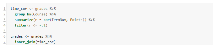
The first scan looks at the linear correlation between when a course was taken (a term number 1-6) and the grade points (0-4.0) for each student who took the course. This entails processing through each course, sub-setting those data points, computing correlations, and then assembling then. Again, this would have take me hours in the old days. Now it's just this:

The script I'm using starts renumbering back at 1 for technical reasons. Lines 1-4 consider the data as grouped by Course, and for each one computes the correlation and stores it in a new variable r. Because we're interested in negative correlations (waiting to take the course associates with lower GPAs), I've filtered to correlations of -.1 or lower. 

Lines 6-7 filter our grade data to just these courses. Now there are seven courses and 3200 data points. Here are the results:


In posting this publicly, I've made the course names generic. They are all STEM or foreign language courses in this case.

Visualization

It's always a good idea to look at the data. Here are the per-term grade averages for the selected courses.

Figure 1. Grade averages by term taken.

I left off the error bars because they cluttered it up. In my first article, I suggested using the year the student took the class, but it's clear here that it's better to use the term number.

Notice the steep decline in Course 8 (pink) over three years. Some of the others, like Course 21 (red) have low GPAs, but they are consistently low.

Models

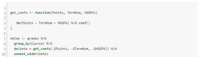
We've now identified some courses where waiting to take them might be detrimental to the student. Another possibility is that the students who wait to take these courses are less-prepared academically. To attempt to disambiguate the waiting effect from the selection effect, we can create a linear model for each course. The dependent variable is average GPA in the course, and the dependent variable is the time the course was taken (TermNum) and the high school grade average (HSGPA). 

Once again we have the challenge of looping over each subject and doing complex calculations, then assembling the results. The tidyverse R packages makes this easy.


Lines 2-5 define a convenience function to build the requested linear model and extract its coefficients. Then we loop over each course with lines 7-8. Line 9 does the work of getting the coefficients. There are three of these, and the do() verb puts them in a list. The last line unpacks the list and turns them into three separate columns.


Notice that of the courses in the selection, number 8 still has a quite significant drop per term in GPA, even after factoring out high school grade averages.

The model for Course 8 has \(R^2 = .13\), which is similar to the correlation coefficient we got earlier (the square root of .13 is .36). It's small but not meaningless. Here are the model details.


Discussion

In the case of Course 8, it is usually taken in the second year, and the effect we see is mostly the difference between years two and three. On the graph, the high numbers for terms 1 and 2 are almost certainly a selection effect--only stellar students take the course that early. The year 2-3 drop raises interesting questions about advising, placement, and preparation. It would be a good idea to redo the analysis using first year college grades rather than high school grades, to see how much effect remains. 

Some of the other courses are worth following up with as well. I didn't include details of each in order to save space here. All in all, this is a successful bit of research that can help specific programs tune their student success pathways. 

If you try this method at your institution and find something interesting, please let me know.

I've had several people ask me for the code to do the grade reliability calculations. It needs some cleaning up before I can post it, but I will try to get it done this week. I want to build the functionality into our custom packages so I easily rerun it, and that takes a little longer than a one-off.