Time to Graduation

How long does it take to complete a bachelor's degree? Furman's four-year graduation rate runs around 75% and the six-year rate is about 81%, so take a guess what the average time to graduation is.

The answer is an average of 3.8 years from start to graduation, a rate that has been steady for years.  Surprised? I was, because the math doesn't seem to add up. Wouldn't it have to be more than four years?

Here's the code I used to calculate time to graduation.

grads <- grads %>%
  mutate(GradDate = ymd(GradDate),
         StartDate = ymd(paste0(Cohort,"/8/20")),
         Time      = as.numeric((GradDate - StartDate)/365.25))

This relies on the lubridate library to convert text strings like "05-07-2021" into a date format and to perform the difference calculation in the last line. Subtracting two dates gives the difference in days, which I divided by 365.25 to get years. I approximated the actual start dates by August 20 of the year they enrolled, which won't be off more than a week (less than 1% of four years). 

The first thing to notice is that August 2016 to May 2020 is three months short of four years, so a "four year graduation rate" is really more like a 3.75-year graduation rate for the majority of our graduates. Additionally, students who take longer than four years, typically do not take longer than five, so a six-year rate is more like a 4.75-year rate in practice.

Using just those two facts we could estimate the time to graduation with 

$$ \frac{3.75(.75) + 4.75(.81 - .75)}{.81} = 3.82 $$

But there are a few three-year graduates too, which brings the average down to 3.8. 

IPEDS has four-, five-, and six year graduates, and the code in the next section can extract such from the CSV files. 

Figure 0. Cumulative graduation rates by quintile of four-year rate.

Just eyeballing the figure shows that lower four-year rates are associated with longer average times to graduation.

Estimating Time to Graduation

As argued in Most college students don’t graduate in four years, so college and the government count six years as “success”, time to graduation is a big deal because it (1) costs money to attend college, and (2) limits the income of the students. It's hard to start a career before finishing the degree, and those extra years are lost earnings and lost experience in the job market.

 

Pundits are already calling curtains for liberal arts colleges, and part of the problem is cost. The benefits of small classes and broad learning goals is a hard sell when a private college costs ten to twenty thousand dollars more per year. But that doesn't factor in the time to graduation! If it takes a year or two longer at a "cheaper" college, that cost needs to be averaged in to make a fair comparison. 

The College Scorecard uses a 200% time to graduation (!), meaning eight years for a bachelor's degree. Fortunately, the IPEDS database has more detailed information, which we can retrieve from the grYYYY tables.

grad_time <- read_csv("gr2019.csv") %>%
  filter(GRTYPE %in% c(8,13,14,15)) %>% 

  select(UNITID,
         GRTYPE,
         N =     GRTOTLT) %>%
  spread(GRTYPE, N, sep = "_") %>%
  mutate(Grad4    = GRTYPE_13 / GRTYPE_8,
         Grad5    = GRTYPE_14 / GRTYPE_8,
         Grad6    = GRTYPE_15 / GRTYPE_8,
         GradTime = (Grad4*3.75 + Grad5*4.75 + Grad6*5.75)/(Grad4 + Grad5 + Grad6)) %>%
  na.omit()

This code snip accesses a local copy of the 2019 IPEDS graduation file (in reality, my code hits a data warehouse instead and averages over three years), and grabs the information about undergraduates who finish in four years or less, five years, or six years. A GradTime estimate follows from that.

 

Figure 1. Estimated time to graduation by institution predicted by four-year graduation rates.

We can estimate the average time to graduation from the four year graduation rate. The regression line is shown in the figure. It's a cubic polynomial in Grad4 and has an R-squared of .81. 

The black line can be used as a cost-scaling factor in addition to a risk assessment. The lower the graduation rate, the riskier it is to enroll because of drop-outs, and on average the longer it will take to graduate as well. I called out two colleges for illustration. St. John's College in Annapolis has a 67% four-year grad rate in the IPEDS survey, and according to  collegeresults.org, has a net cost of about $30K/year. Youngtown State University, in Ohio, has a net cost on the Scorecard of about $12K/yr, and a four-year graduation rate of about 19%.

Note that the y-axis isn't zeroed, which makes the gap seem larger than it is. The time-to-graduation difference between these two schools represents about an 18% extra cost for YSU graduates due to the extra time to graduation, so a comparative yearly cost of $14K instead of $12K. This doesn't count opportunity cost--the lost earnings from being in a job earlier--so it's a conservative estimate.

Career Lag

The analysis so far is unsatisfactory because it doesn't consider the fates of students who do not graduate. I'll illustrate how this might be done. Students who do not graduate may transfer to another college and finish there, or may drop out. Either way, it sets them behind because of lost time and credits. For the sake of argument, assume that the resulting career lag penalty for dropping out of the first school attended is ten years. A normal lag is 3.75 years--the time a first-time full-time freshman takes to earn a bachelor's degree if all goes as planned. For non-graduates, this hypothetical extra lag is intended reflect the earnings penalty for not getting the diploma, or having to wait because of transfer mechanics. Its a guess--don't take it too seriously.

The formula for career lag is then

CareerLag = (Grad4*3.75 + Grad5*4.75 + Grad6*5.75 + (1-Grad4-Grad5-Grad6)*nongrad_career_lag) # nongrad_career_lag = 10

We can run the same analysis as before to get the graph below.

Figure 2. Hypothesized career lag by institution predicted by four-year graduation rates.
 

This model has an R-squared of .91; you can see it's pretty linear. Now the difference between the two highlighted schools is more than a 30% difference. We will get different values if we pick different non-grad penalties.

Discussion

I'm not that familiar with the labor economics work in higher ed. Brian Caplan's book has a nice primer, but I don't recall that much about time to graduation. A quick google turns up these related articles:

• Delayed Graduation and Over-education
• Does Time-to-Degree Matter?
• Delayed Time-to-Degree and Post-college Earnings 
  

My scan of these suggests that the situation is complicated (e.g. are students working while in college, explaining the delay to graduation?), but that taking longer to graduate is associated with lower earnings, and that this may be partly due to signalling to the labor market. Students who take longer to graduate may be seen as less capable.

In 2020, Sara Vanovac and I published a validity analysis of student writing assessments and discovered a Matthew effect wherein students with the highest levels of assessed writing ability were also seen to develop the most quickly. We went looking for other examples of this type of divergence and found one in Raj Chetty, et al's work on equality of opportunity. 

Here's figure 8 from our paper, showing an inter-generational divergence in earnings.

Figure 3. Selectivity of universities of children is associated with incomes of parents. Right: incomes of children who graduate is linked to the selectivity of the institution.

The figure uses the mammoth data set Chetty scoured from tax records to suggest that lower incomes persist despite college opportunity partly because of the effect of college selectivity (which includes the type of students they select). The incomes for those attending non-selective institutions barely exceed parent incomes--for those who graduate. This may be partly due to longer graduation times. The figure doesn't take into account the reality that lower selectivity entails lower graduation rates as well, so the true picture on the right is more divergent that the one shown.

Conclusions

We can add time to graduation to the list of student success measures we track, like retention and graduation rates. I've started using four-year rates for bachelor's programs, instead of the more common six-year rates, as a proxy for institutional quality (outcomes for students).

It may be that delaying graduation is beneficial to a student, for example working to pay for college in a job that benefits their career. There's no way to know without studying the matter at your institutions: what types of students leave before graduation and what types of students take longer to graduate? Are these the same groups? With data from the National Student Clearinghouse we can calculate time to graduation for transfer-outs (and transfer-ins).

Resources

The code I used to make the first two figures is here. You can modify it to read CSV files downloaded from IPEDS if you don't have those tables in a database.

Updates

After the initial post, I went back and added Figure 0. The github code is updated too.

Delay Time Code and Example

Introduction

Last time I sketched a research idea to examine the link between when students take a course and their grades in the course. This is particularly applicable to gateway-type courses either in general education or in popular majors. This time I'll show show some code and talk about real results.

I haven't found a great way to embed code, so I used images. I apologize for that, but this isn't really copy/paste-able anyway, due to the customization to our specific circumstances. 

Getting the Data

In my experience, getting data and preparing it for analysis is time-consuming. In the old days of Excel and SPSS, it was prohibitive. I remember printing out multi-sheet correlation tables, taping them to the wall in a big grid, and manually highlighting them. Or importing CSV files into Access so I could run SQL queries to join them. Thankfully, those days are over.

We've spent a lot of effort to streamline data access so we can spend more time doing statistics. All the data comes from our IR data warehouse, and we use R's library(odbc) with library(tidyverse) to accomplish the rest. This just requires setting up a local ODBC connector on your machine. Once the connection (called dbc for database connector) is in place, getting data is easy.

Lines 1-7 below join the CourseEnroll table with the CourseSections table. The first has grades for each student, keyed by a SectionID, adn the second has information about that course. Specifically we want the subject code and number, e.g. BIO 101.

The select statement is actually a dplyr verb, not an SQL command, but it gets translated in the background to SQL to make the query. This is a huge time-saver, because I don't have to mix SQL and R code. It's also easy to read. 

By line 9, we've connected two tables and are set up to pull course names (e.g. BIO 101). Lines 9-15 specify what we want to pull down from the two tables: the student ID, the term the course was taken, the letter grade, the course points and credits, and the subject and number of the course. 

I decided to ignore withdrawals, although that might be interesting to study too. So lines 17-19 filter the data to courses with credit that have an A-F grade, and are relatively recent. 

The collect() verb tells R to pull all this down from the database. So in the background all the code in lines 1-19 gets translated into one big SQL statement, which is now executed. 

Lines 23-24 go back to the database using a convenience function we have in a custom package, to retrieve all students who are in our official first-time full-time freshmen cohorts. Since we want to understand sequential course-taking, it makes sense to exclude transfers and other sorts of students.

The most recent returning class (entering fall 2017) hasn't had two full years yet, so I excluded those in line 25. That leaves us cohorts 2012 through 2016 as data points.

Line 27 uses another custom function to add the start term to each student record. This is inefficient computationally, but easy to add here since I had the function handy. The start terms should all be the fall of their cohort year, and that would be another way to do it, using mutate() and paste().

Now we need to tweak the data a little.

The mutate() verb in dplyr lets you create new columns or change existing ones. Here, I use a custom function to compare the term each course was taken with the student's start term to find the time elapsed. This returns a number 1,2,3..., where 1 means first fall/spring term attended, and so on. There are a very few odd cases where it might turn out to be zero, so I round those up in line 30. 

We want to study courses taken early in a student's career, so any terms after 6 (end of junior year) I round down to 6. There aren't many cases like that, and it cleans up cluttered cases with small Ns.

Line 32 fixes a change in course prefixes that happened a couple of years ago, to make them match across time. 

Line 33 creates a Course variable by combining the subject and number, e.g. "BIO" and "101" turn into "BIO 101".

Finally, line 34 calculates the grade points assigned, where 4.0 = A, 3.0 = B, etc. 

Lines 36-38 look at the admissions data table and retrieve high school grade averages, which have been recalculated to be on a common 4-point scale. 

In the pre-R days, this data assembly probably would have taken me half a day. Now it just takes as long as writing the description and fixing typos and logical errors. Most importantly, the process is standardized and transparent. It runs in a few seconds, even through VPN. 

The result is about 57,000 data points, illustrating the comparison with formal assessment data. As someone once said, quantity has a quality of its own. 

The Research Data

Now that we have courses and grades, coupled with when students took the courses and their high school grades (to use as a predictor), we can narrow the data down to the courses that are the focus of the research. In this instance we only care about courses that are commonly taken by students in their first two years of college.

The filter in line 42 says we only care about the first two years. The next line counts total enrollment for each course and calls that count N_enroll. Line 44 sorts the list so it's easy to scan when printed out, and line 45 filters courses to those with at least 200 students enrolled. That list of courses is saved in a new data frame called popular_courses.

Lines 47-48 inner join the popular courses with the grades data, meaning only the courses in the former are now in the data set: 37 courses and 18,000 data points.

Correlations 

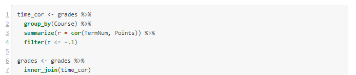
The first scan looks at the linear correlation between when a course was taken (a term number 1-6) and the grade points (0-4.0) for each student who took the course. This entails processing through each course, sub-setting those data points, computing correlations, and then assembling then. Again, this would have take me hours in the old days. Now it's just this:

The script I'm using starts renumbering back at 1 for technical reasons. Lines 1-4 consider the data as grouped by Course, and for each one computes the correlation and stores it in a new variable r. Because we're interested in negative correlations (waiting to take the course associates with lower GPAs), I've filtered to correlations of -.1 or lower. 

Lines 6-7 filter our grade data to just these courses. Now there are seven courses and 3200 data points. Here are the results:

In posting this publicly, I've made the course names generic. They are all STEM or foreign language courses in this case.

Visualization

It's always a good idea to look at the data. Here are the per-term grade averages for the selected courses.

Figure 1. Grade averages by term taken.

I left off the error bars because they cluttered it up. In my first article, I suggested using the year the student took the class, but it's clear here that it's better to use the term number.

Notice the steep decline in Course 8 (pink) over three years. Some of the others, like Course 21 (red) have low GPAs, but they are consistently low.

Models

We've now identified some courses where waiting to take them might be detrimental to the student. Another possibility is that the students who wait to take these courses are less-prepared academically. To attempt to disambiguate the waiting effect from the selection effect, we can create a linear model for each course. The dependent variable is average GPA in the course, and the dependent variable is the time the course was taken (TermNum) and the high school grade average (HSGPA). 

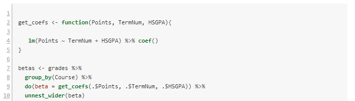
Once again we have the challenge of looping over each subject and doing complex calculations, then assembling the results. The tidyverse R packages makes this easy.

Lines 2-5 define a convenience function to build the requested linear model and extract its coefficients. Then we loop over each course with lines 7-8. Line 9 does the work of getting the coefficients. There are three of these, and the do() verb puts them in a list. The last line unpacks the list and turns them into three separate columns.

Notice that of the courses in the selection, number 8 still has a quite significant drop per term in GPA, even after factoring out high school grade averages.

The model for Course 8 has \(R^2 = .13\), which is similar to the correlation coefficient we got earlier (the square root of .13 is .36). It's small but not meaningless. Here are the model details.

Discussion

In the case of Course 8, it is usually taken in the second year, and the effect we see is mostly the difference between years two and three. On the graph, the high numbers for terms 1 and 2 are almost certainly a selection effect--only stellar students take the course that early. The year 2-3 drop raises interesting questions about advising, placement, and preparation. It would be a good idea to redo the analysis using first year college grades rather than high school grades, to see how much effect remains. 

Some of the other courses are worth following up with as well. I didn't include details of each in order to save space here. All in all, this is a successful bit of research that can help specific programs tune their student success pathways. 

If you try this method at your institution and find something interesting, please let me know.

I've had several people ask me for the code to do the grade reliability calculations. It needs some cleaning up before I can post it, but I will try to get it done this week. I want to build the functionality into our custom packages so I easily rerun it, and that takes a little longer than a one-off.