Showing posts with label prediction. Show all posts

Thursday, November 07, 2019

Variable Selection for Predictive Models

Not so long ago, if you had a list of potential explanatory variables \(X\) to use to predict some output \(Y\), you'd ask the software to start somewhere and interatively build regression models to test the combination of variables. Often, the coefficients of \(X\) that had small p-values were kept and the others discarded. This step-wise approach has detractors, and there are methods available now that are recommended by people who should know. In particular, I recommend Regression Modeling Strategies by Frank Harrell.  In this post I'll demonstrate the use of one of the recommended replacements for step-wise variable selection.

Scanning \(X\)

In institutional research we often have dozens or hundreds of potential explanatory variables. For example, using The Freshman Survey to predict first year attrition gives us over a hundred data points for responders. I like to scan them quickly using AUC to see which ones are interesting, and built a tool to do that. You can find Survey Prospector on github here, with links to show how to use it. 

For the Titanic data, I'll just loop through the variables and compute the AUCs in order. To do this, the Sex variable needs to be converted to a number, so I turned it into Male, a dummy variable (1 = male, 0 = female), and added an interaction PclassM = passenger class times male status. 

Variable AUC
Survived 1.00
PclassM 0.80
Male 0.77
Fare 0.69
Pclass 0.68
Parents/Children Aboard 0.56
Siblings/Spouses Aboard 0.54
Age 0.52

The first entry just shows that the output variable Survived can predict itself perfectly. Surprisingly, Age isn't helpful at all, with an AUC barely above the guessing rate of .50.

This table is helpful in orienting us to which are the useful inputs, but this approach has two blind spots:
  • The AUC is agnostic as to the shape of the relationship between the explanatory and predicted varaibles: it's not a measure of a model quality. So we don't know if the relationship is linear, quadratic, etc. All we know is that it's an ordered relationship, so that higher values (lower if the scale is reversed) of the predictor mean higher probabilities of survival on average, when AUC > .5--measured in the sense already described, where we have to distinguish between the two cases.
  • The list of AUCs doesn't tell us anything about the correlational structure of the predictors. There's a tab in SurveyProspector for that, or we can run a correlation table to help. I'll skip that step here.

Model Selection

We have a sense of which variables are important. If the list was really long, we could now weed out the ones that aren't likely to be useful--at least for most purposes in higher education. It's possible that a variable with a low AUC happens to have an important interaction with some other variable, but I haven't come across a case like that in practice.

This leaves us with the problem of which of the "good" inputs to include in the model. Step-wise regression was supposed to solve this problem, but it turns out to have problems. With seven inputs, there are \(2^7 = 128\) possible models. One method is just to check all of them and use some metric for model selection. This is perilous, because we'll probably over-fit the data. 

The approach I'll demonstrate here uses a penalization term on the regression equation. It's similar to Lagrange multipliers, if you're familiar with that optimization technique. Every coefficient of \(X\) has to earn its keep, enforced by adding an artificial "error term" that adds in a multiple of the coefficient values. In order to make the total error decrease, the optimizer tries to keep the coefficients small (starting at zero). There are variations, including LASSO and ridge regression. I'll show off LASSO here. They differ only in how the extra error term is calculated.

Model error as number of variables increases (read right to left)


Reading the graph above from the left, it shows the effect of adding more variables to the model. The idea is to find a good trade-off between the number of variables (smaller is better) and smaller error. The dashed line at 4, with log(Lambda) close to -4, is a good compromise. The lambda is the penalty term that adds the extra error to be optimized away. It decreases as we move to the left, until we end up a ordinary regression with no extra error.
Model coefficients as number of variables increases (read right to left)


The corresponding graph of variable coefficients tells us which variables are important for each model we could choose from the menu. With four inputs (degrees of freedom, one of which is the regression constant), at log(Lambda) about -4, it looks like the variables included are Male, Pclass, and Sibs, but we can actually retrieve the coefficients and see more exactly:


We can leave off Fare, since it's coefficient is so close to zero. Age is also not very important.

The model's ROC curve is plotted below.

ROC curve for the LASSO model with log(lambda) = -4

R Code


library(tidyverse)
library(glmnet)
library(plotmo)

x <- pass %>% 
  select(Pclass,Sex,Age,Fare, Sibs= `Siblings/Spouses Aboard`, Child = `Parents/Children Aboard`) %>% 
  mutate(Male = (Sex == "male") + 0,
        PclassM = Pclass*Male) %>% 
  select(-Sex) %>% 
  as.matrix()

y <- pass$Survived

# glmnet(x,y) has inputs in matrix x and output in y
my_fit <- glmnet(x, y, alpha=1, family="binomial")

# graph it
plot_glmnet(my_fit, xvar="lambda", label = 10)

# print the coefficients
coef(my_fit, s = exp(-4))

# cross validation
plot(cv.glmnet(x, y, alpha=1))

# predictions
p <- predict(my_fit, x, s = exp(-4)) 

# we have to do the inverse transform for the logit
p <- 1/(1 + exp(-p)) 


Tuesday, November 05, 2019

Stories from Data


In the last few articles I explored the meaning of the AUC metric for predictor performance. Let's take it for a test drive with a model of Titanic survival that involves more than passenger class.

Using R's general linear model, we can create a binomial predictor of survival with one line:

logistic_model <- glm(Survived ~ Pclass*Sex + Age, family = "binomial", data = pass)

This model assumes that passenger class and sex of the passenger will interact, and that age is important. It's like "women and children first, starting with the wealthy."

Here's the output.

Estimate Std. Error z value Pr(>|z|)
(Intercept) 7.7418 0.9256 8.36 0.0000
Pclass -2.3054 0.3089 -7.46 0.0000
Sexmale -6.0872 0.8900 -6.84 0.0000
Age -0.0355 0.0074 -4.82 0.0000
Pclass:Sexmale 1.3975 0.3260 4.29 0.0000

This is an old-fashioned way to examine model parameters, by looking at p-values. In that mode of thinking, if the p-values are near zero it means that the actual coefficient in question probably isn't zero. In this case, it says that all the coefficients are non-zero. In particular, the interaction between class and sex turned out to be important. You can see that Sexmale has a large negative coefficient, meaning men were at greater risk. to a lesser extent, the passenger class 1,2,3 increases risk as well. Putting those two things together, we actually take back a little of the risk for the men as the passenger class increases, since the interaction Pclass:Sexmale is positive. 


ROC graph for the predictive model


The shape of the ROC graph shows that we can easily predict half the survivors using this model, since the graph zooms up to about .5 before turning to the right. 

When we only considered passenger class, we made a matrix showing the conditional probabilities of class 1,2,3 given the survival state. In the current model, the predictor has too many unique values to make a table like that, but we can make a graph instead. Imagine turning the table on its side and plotting the two values (survived or not) in different colors.

The x-axis shows the modeled probability of survival, with blue being actual survivors.


At the far right, the probability of survival per the model is very high--near 100%--and the actual rate of survival there is much higher (blue) than the non-survivors (pink overlap). At the left end of the graph, the predicted probability of survival is near zero, and there's a large bulge of non-survivors there. This separation is a sign of a good predictor. If the blue and pink areas overlap, the predictor isn't distinguishing cases very well.

The Story

So far all of this is just rows of data arranged in different ways, but there were real people behind each of them. What if we ask this question: who should have survived, but did not?

In the last graph, we can see that there are a few passengers with high probabilities of survival (far right), who perished. Who are they?

Here's the query.

pass$Probability <- fitted.values(logistic_model) # append the original data with computed probability of survival
pass %>%                                          # use passenger data with probabilities appended
  filter(Survived == 0) %>%                       # filter to only non-survivors
  arrange(desc(Probability)) %>%                  # sort by probability of survival in descending order
  select(Name, Sex, Age, Pclass, Probability) %>% # pick the most useful fields to look at
  head(10)                                           # get the first ten of them

And the output.

Name Sex Age Pclass Probability
Miss. Helen Loraine Allison female 2 1 0.9953459
Mrs. Hudson J C (Bessie Waldo Daniels) Allison female 25 1 0.9895226
Miss. Ann Elizabeth Isham female 50 1 0.9749029
Miss. Henriette Yrois female 24 2 0.9070513
Mrs. William (Anna Sylfven) Lahtinen female 26 2 0.9008834
Mrs. William John Robert (Dorothy Ann Wonnacott) Turpin female 27 2 0.8976647
Miss. Annie Clemmer Funk female 38 2 0.8557757
Mrs. Ernest Courtenay (Lilian Hughes) Carter female 44 2 0.8274153
Mrs. (Mary) Mack female 57 2 0.7512785
Miss. Ellis Anna Maria Andersson female 2 3 0.6801742

Notice that the first two names on the list, with the highest probabilities, share the last name. Since the Titanic is so famous, there are whole sections of the Internet devoted to information about passengers. Here's the heart-breaking story of Bess Allison. 

This example vividly shows the uncanny insights that can be obtained through careful data analysis.

Since I called the p-value approach "old-fashioned" earlier, next time I'll describe the new-fashioned version.

Sunday, November 03, 2019

AUC Calculations

Introduction

In the last post on this topic, the AUC metric of classifier performance was seen to have a dual nature. It can be viewed as a probability calculation or the area under a particular curve (AUC = area under curve). These are mathematically equivalent, and the basic principle behind both is easy to understand and useful to know.

Recall that we want to distinguish a "success" case \(Y_1\) from a "failure" case \(Y_0\), based on some information we have about each case, \(X_1\) and \(X_0\). Unless the scale is reversed, we compare the two predictors and guess that \(Y_1\) is the one with the greatest value of \(X\). If there is a tie, we have to flip a coin.

The explanatory power of a predictor in these conditions derives from

$$( Pr[Y_1 | X_1 > X_0] - Pr[Y_0 | X_1 > X_0] ) /2.$$

That is, we take the probability that the predictor gives us the correct answer and then subtract the probability that it gives us the wrong answer. On the ROC graph, this probability difference is the area above the diagonal guessing line. 

Titanic Example

The distribution of passenger class is different for survivors and non-survivors. The rates are
$$ \begin{matrix}
Pclass & Y_0 &Y_1\\
1 & 0.147 & 0.398\\
2 & 0.178 & 0.254\\
3 &  0.675 & 0.348\\
\end{matrix}$$

For example, for a randomly-selected survivor \(Y_1\), the probability of being in first class is about 40%, but for a non-survivor it's only 15%. So when a random selection is made from each of these columns to pick a \(Y_1\) and \(Y_0\), the combined probabilities are obtained by multiplying out each of the possibilities. See the R code at the end for how to do this. The result is a square matrix

$$\begin{matrix}
 & & & Y_0 \\
&  & Class1 & Class2 & Class3\\
& Class1 & 0.058 & 0.071 & 0.269\\
Y_1 & Class2 & 0.037 & 0.045 & 0.172\\
& Class3 & 0.051 & 0.062 & 0.235\\
\end{matrix}$$

showing for example that the joint probability of the survivor \(Y_1\) being in first class and the non-survivor \(Y_0\) being in third class is 26.9%.

We will correctly classify the two cases (guessing which one of the two is \(Y_1\)) only when the passenger class is greater for \(Y_1\), or if the two classes are the same and we guess correctly. To reflect this correct probability rate for each of the entries in the matrix above, we can weight them accordingly to obtain

$$\begin{matrix}
  & Class1 & Class2 & Class3\\
Class1 & 0.029 & 0.071 & 0.269\\
Class2 & 0.000 & 0.023 & 0.172\\
Class3 & 0.000 & 0.000 & 0.117\\
\end{matrix}$$

The entries above the diagonal haven't changed, and the ones on the diagonal (where the classes are equal) have been halved, since we have to flip a coin in those cases. Below the diagonal, the predictor is giving us the wrong answer: the passenger class of the survivor is lower than the non-survivor, so those cells are zeroed out--they don't add to the probability of being correct.

We can obtain the AUC by simply adding up the probabilities in the last matrix, to get .68. Here' the ROC graph.

ROC graph for passenger class predicting survival

Improvement Over Guessing

The computation above gives us the whole AUC, which includes the cases in which we just guess correctly. Notice that the diagonal of the last matrix sums to only about 17%, far less than the 50% rate we can get by ignoring passenger class and just flipping a coin. 

To get the excess probability over guessing, which in our case is .68 - .50 = .18, we have to use the formula advertised at the top, viz: for each combination of passenger class, like 1 vs 2, find the probability that we get the right answer and subtract the probability that we get the wrong answer and divide by two. That matrix, after dividing by two, looks like

$$ \begin{matrix}
  & Class1 & Class2 & Class3\\
Class1 & 0.000 & 0.017 & 0.109\\
Class2 & -0.017 & 0.000 & 0.055\\
Class3 & -0.109 & -0.055 & 0.000\\
\end{matrix} $$

We only care about the upper triangle here, above the diagonal, which is .017 + .109 + .055 = .180. (The entries below the triangle just tell us what would be the case if we had our predictor reversed: we'd get an AUC less than .5 by .18).

The steps in the calculation of the excess probability are the same as finding the area of a triangular region, which is one way the AUC can be calculated. The comparison is shown in the areas in the image below.


[Edit] Why Divide by Two?

The divide-by-two in the formula may seem mysterious. Here's where it comes from. I'll demonstrate for the 2x2 case. The general result comes from the same idea.

If we go back to our column-normalized matrix 

$$ \begin{matrix} & Y = 0  & Y = 1 \\ X = 0 & a & b \\ X = 1 & c & d \end{matrix} $$

and multiply columns (outer product of the second column with the first), we get the probability of each possibility:

$$ \begin{matrix} ab & bc \\ ad & cd \end{matrix} $$

The predictive power comes from the \(ad\) case, where the values of \(X\) are in the correct direction to pick \(Y = 1\). As we saw before, 

$$ AUC = ad + \frac{1}{2}(ab+cd) $$

where the second term is due to guessing when the predictor values are the same for both cases. The algebraic trick we need is the fact that the second matrix above sums to 1, so that we could also write 

$$ AUC = 1 - bc -  \frac{1}{2}(ab+cd) $$

Then we just add the two AUC formulas and divide by two to get

$$ AUC = \frac{1}{2} + \frac{1}{2}(ad-bc) $$

The explanatory power beyond guessing is what we get after subtracting the 1/2. In the general case, we have to sum up all the pieces that look like \(ad-bc\), which amounts to taking the probability matrix, subtracting its transpose, summing anything above the diagonal, and dividing by two.

This, in turn, is just an application of a kind of probabilistic "recentering around .5" you can do with any event A. If A' is the event's complement, then

\( Pr(A) = 1 - Pr(A') \) so \(2 Pr(A) = Pr(A) + 1 - Pr(A') \), or

$$ Pr(A) = \frac{1}{2} + \frac{1}{2}(Pr(A) - Pr(A')) $$

The direct summing of probabilities in the frequency matrix is the left side of the equation. The summing of triangles in the geometric AUC calculation is the right side.

R code

library(tidyverse)
library(knitr) # optional -- pretty tables

# read in data 
pass <- read_csv("titanic.csv")

# calculate the passenger class frequencies conditional on survival status
rates <- pass %>% 
  select(Y = Survived, Pclass) %>% 
  group_by(Y, Pclass) %>% 
  summarize(N = n()) %>% 
  mutate(P = N /sum(N)) %>%
  select(-N) %>% 
  spread(Y, P, sep = "_")

# print out the matrix
rates %>% kable(digits = 3, format = "latex") %>% cleaner()

# create the matrix of probabilities for class combinations for Y0 and Y1
class_prob <- outer(rates$Y_1, rates$Y_0) 
rownames(class_prob) <- colnames(class_prob) <- c("Class1","Class2","Class3")

# print out the matrix
class_prob %>% kable(digits = 3, format = "latex") %>% cleaner()

# when X1 > X0 the weight is 1. When x1 = X0, we have to guess, so the weight is .5. 
# when X0 > X1 we'll get the wrong answer, so its weight is zero
case_weights <- upper.tri(class_prob) + 0 
diag(case_weights) <- .5 # classes match, so guess

# print out the matrix
(class_prob*case_weights) %>% kable(digits = 3) 

# compute the AUC
sum(class_prob*case_weights)

# compute the explanatory power in excess of guessing
prob_diff <- (class_prob - t(class_prob)) / 2

# print it
prob_diff %>% kable(digits = 3)

sum(prob_diff[upper.tri(prob_diff)]) 

Thursday, October 31, 2019

ROC Example

Introduction

The discussion of binary predictors (e.g. retain/attrit) so far has focused on the AUC measure of an independent variable's power to predict the outcome. As with any performance measure, we have to make assumptions and then live with the consequences. In this case, we set the question up in a rather artificial way: we assume that we have to choose between two cases \(y_0\) and \(y_1\), where the first case has outcome 0 (e.g. a student who failed to return, if predicting retention), and the second case has the outcome 1 (e.g. a student who did return). The job of the independent variable \(x\) is to distinguish which case is which. This is a different task than taking all the \(x_i,y_i\) pairs of data and, for example using regression to minimize error. Regression models have other kinds of performance measures, although we can use AUC for a logistic (i.e. binary) regression. See Frank Harrell's blog for some commentary from an expert.

Despite its limitations, I find AUC useful for scans of predictors and for communicating to non-technical audiences. It's much easier to explain the "guess which" scenario than regression goodness of fit measures. So the purpose of this post is to delve into AUC and its dual nature as a probability interpretation and a geometrical one. Last time I claimed that AUC was:

  • The probability of distinguishing \(y_0\) from \(y_1\) when given the explanatory variable \(x\)
  • The area under the ROC curve.
It is by no means obvious that these two things should be the same, so I'll use the 2x2 case to show it's true in the simplest case. We already know that the outcome only takes values 0 or 1, and in this simple case, the explanatory variable also only has 0 or 1 value. For example, if you want to use "early admit" status to predict first year retention, both variables are binary. I'll continue to use that case as an example for concreteness. 

Preliminaries

Start with what is called the "confusion" matrix, where we take historical data and populate the four possible outcomes of the predictor

$$  \begin{matrix}  & y = 0 & y = 1 \\  x = 0 & A & B  \\ x = 1 &  C & D  \end{matrix} $$

with frequencies of occurrence. Here, \(A\) is the fraction of all cases in the data where the predictor  is zero (i.e. not early admit) and the outcome was zero (student did not return for second year). 

Recall that the setup for the AUC calculation is that we assume a random draw has occurred to choose a case where \(y = 0\) and a case where \(y = 1\). That means we need to condition the confusion matrix by dividing by the column sums to obtain conditional probabilities:

$$  \begin{pmatrix}    \frac{A}{A+C} & \frac{B}{B+D}  \\  \frac{C}{A+C} & \frac{D}{B+D}  \end{pmatrix} := \begin{pmatrix}    a & b  \\  c & d  \end{pmatrix},$$

where for convenience I've renamed the normalized values with lowercase letters. Now we can proceed to compare the probability and area interpretations of AUC.

AUC as Probability

Suppose we are presented with two cases, and we know that one of them has \(y=0\) and the other has \(y=1\). If our predictor is any good, then \(x = 1\) should associate more with \(y=1\). It's also possible that the predictor is reversed (as in negatively correlated), but that just entails reversing the direction. For example, if we used first generation status to predict retention, we would probably find that those students had lower retention, so we would need to change the semantics of the predictor to NOT first generation student to get the two variables to positively correlate. That's just for convenience in interpretation. 

Assuming \(x\) is useful, we'll then predict that if one case has \(x = 0\) and the other case has \(x = 1\) that the second case is more likely to be the \(y=1\) case. In the example, if we are given a student who is early admit and one who is not, we'll assume it's the former who returns the next year. 

When the random draw of the two cases is made, the probability that  \(y_0\) has \(x = 0\) is \(a\) in the matrix, and the probability that  \(y_1\) has \(x = 1\) is \(d\), so the probability that both happen independently is the product \(ad\). Similarly, the probability that our predictor gets is exactly wrong is \(bc\), and the probability of a tie (both cases are early admit or both are not) is \(ab + cd\). In the case of a tie, we just have to guess, so the probability of a correct answer is one half.

This gives us a probability of correct classification of $$ \begin{align} ad + \frac{1}{2}(ab + cd) & = \frac{2ad + ab + cd}{2} \\  & = \frac{a(b+d) + d(a+c)}{2} \\ & = \frac{a + d}{2} \end{align},$$

where the last step comes from using the definition of the lower-case variables (convert back to the capital letters to see it).

In the language of classifiers, \(a\) and \(d\) are called the True Negative Rate (TNR) of classification and True Positive Rate (TPR). So the AUC is the average of the two in the 2x2 case. 

AUC as Area

The Receiver-Operator Characteristic (ROC) curve plots the False Positive Rate (FPR) on the horizontal axis and the TPR on the vertical axis, where TPR = 1 - TNR. The fourth variation on this theme is the False Negative Rate (FNR). Putting these names on our matrix, we have

$$ \begin{matrix} a = TNR & b = FNR \\ c = FPR & d = TPR \end{matrix} $$

The ROC graph looks like this:


ROC curve for our binary classifier.

The most satisfying way to find the area of a polygon is to use this formula, whereby we get a list of points to traverse counter-clockwise, starting and ending at (0,0).

$$ \begin{matrix} 0 & 0 \\ 1 & 0 \\ 1 & 1 \\ c & d \\ 0 & 0 \end{matrix} $$

Cross-multiplying, summing, and dividing by two (see the link for details) gives \( (1 + d - c)/2 \), which is the same as \( ( a + d) /2 \), as we got before. 

Discussion

The illustration shows that for a binary predictor and a binary outcome, the probability of correct classification is the same as the area under the ROC curve, and that both are equal to the average of the true positive and true negative rates. Under more general conditions, it is still true that the probability and the area are equal. The TPR and TNR are not defined in that case--they specifically refer to the 2x2 version. 

There are other statistical connections we can make to AUC, and the blog post linked above does some of that. For the 2x2 case, we have

$$ \begin{align} Var(X) &= (A + B)(C + D) \\ Var(Y) &= (A + C)(B + D) \\ Cov(X,Y) & = AD - BC \end{align} $$

If you compute how much area in the ROC lies above the "guessing" rate (the line from (0,0) to (1,1)), you find it's \( ad - bc \), which is the covariance divided by both variances. This is almost the definition of the Pearson correlation between the predictor and outcome variables. 


Monday, October 28, 2019

ROC and AUC

This post continues the previous topic of thinking in predictors. I showed a measure of predictiveness, called AUC, which can be thought of as the probability of correctly guessing which of two different outcomes is which.Here I'll show how to visualize predictive power and relate the graph to that probability.

Suppose we want to predict which students will do poorly academically in a gateway course, where we define that by the student receiving C, D, or F. If we can predict that outcome far enough in advance, maybe we can do something to help. Note that this is a binary outcome (i.e. binominal), meaning there are only two possibilities.

The predictors we might consider are class attendance, use of tutoring services, prior grades, etc. I'll use the first two of these as illustrations. For example, back to the cups of the prior post, suppose one cup has the ID of a student who earned a C, D, or F, and the other cup has the ID of a student who earned an A or B. You don't know which cup is which, but you are told that the student on the left came to class all the time, and the one on the right did not. You'd probably guess that the one on the left is the A/B student. The probability of that being correct on average is what I called AUC.

You can find many explanations of ROC curves and AUC online, but I find the following twist on it easier to understand.

Imagine that we have all our historical students listed in a spreadsheet, along with all the information we need to know about each in order to assess predictors. We need to know their course grade, and we need to know whatever information is potentially predictive of that grade. The grade will separate students into the sought group (CDF) and the ones who don't need help (AB). Any subset of the students will have a percentage of CDF and a percentage of AB students. We can visualize all possible subsets of students by plotting these as y and x.

Visualization of possible subsets of students

For example, the top right corner of the box contains 100% (all the way to the top) of the CDF students, and 100% (all the way to the right) of the AB students. That subset is the set of all students. At the bottom left, we have 0% of each, or no students--the empty set. If we had a perfect predictor, it would allow us to find the top left "pure" CDF subset just from the predictive information.

Randomly select half the students
Note that the number of students in each category (CDF versus AB) do not have to be equal, because we are using the percentage of each category separately. I put sample Ns on the figure above. Imagine that we randomly select half the students as our "predictor" of which ones will be CDF. On average, we'd expect to get half of the total in each type (i.e. 15 of the 30 CDFs and 50 of the 100 ABCs). The red lines indicate 50% of each of the AB and CDF students (50 and 15, respectively). The point representing a 50% random selection of students is in the center of the diagram.

All random selections are on the diagonal on average

If we randomly chose 10% or 60% of the students instead of 50%, we'd still be on the diagonal, just lower to the left or higher to the right, depending on the percentage. Any random selection results on average in a subset represented by a point on the red line above. This is a handy reference line, because anything above that line means that the percent of CDF students is greater than random--this is what we want in a predictor.

Students who don't come to class

Now consider our possible predictors. Assume for the sake of illustrate that when we look at the group of students who rarely (or never) come to class, that ALL of them are in the CDF category. There are not very many of these students, maybe just 20% of all the CDFs, but this information is good to know. The green X marks the spot on the diagram that represents the subset of students who rarely/never come to class. Notice that the line from the bottom left empty set goes straight up toward the set at the top left, which is just CDF and no AB students (the ideal set we could find with a perfect predictor).

Adding information about students who don't use totoring
Now we can add more information we know about students. The next segment of the green line assumes that any student who does not come to class gets classified as CDF, and in addition we will classify any student who doesn't attend tutoring also as CDF. The combination of these two rules results in the second green X.

Notice that the slope of the line from the first X to the second is not vertical like the first line segment was. The new rule about tutoring is not nearly as good a predictor, because it's moving to the right, meaning that it includes AB students as well as CDF students. That's probably because some AB students don't need tutoring. However, the slope of the second line segment is still steeper than the red guessing line, meaning that the tutoring rule (no tutoring => CDF) is still better than random selection. The graph makes it visually easy to see this.

In practice, after doing this analysis, we might decide to start with the students who aren't attending class, to see if we can solve that problem. It's inefficient to try to help students who don't need it, which makes the use of a predictor an economic decision, not just a mathematical one.

Graphs of this type are called Receiver-Operator Characteristics curves, for historical reasons, and AUC stands for "area under the curve." Next time, I'll explain why this area and the probability we started with are the same thing.

Example: Surviving the Titanic

The passenger list from the Titanic, annotated with survival information, has become a common data set for prediction and machine learning exercises.
Titanic survivorship by passenger class
The graph shows a ROC curve using passenger class as a predictor of survivorship. The circled 1 shows us where the first class passengers are as a subset of all passengers. They comprise a little more than 40% of the passengers who survived (vertical axis), but less than 20% of the ones who died. Notice that the slope of the first line segment is significantly higher than the random selection line in red.

If we guess that all first class passengers will survive, and further assume that all second class passengers will too, we end up at the 2 on the diagram. Notice that the slope of the segment from 1 to 2 is better than random selection (the red reference line), but not by that much. If we also include 3rd class, we end up with all the passengers. Notice that the slope of the line from 2 to 3 is significantly less steep than the reference line--meaning the odds of surviving as a 3rd class passenger are worse than random selection from all passengers.

Quiz

Test your understanding with the questions reference the figures below.
Answer the questions below

Questions:
  1. Which of these predictors has the highest probability of correct classification?
  2. Which has the lowest?
  3. Which of (a) and (d) would be preferred for a small intervention program?
Scroll down for answers.


Answers:
  1. c has a curve that gets closest to the top left perfect prediction subset, and if you imagine the area being shaded under the green line, it's larger than any of the others.
  2. b is indistinguishable from random selection
  3. We prefer d because it initially goes straight up, meaning we can select a small treatment group with little error.


Sunday, October 27, 2019

Thinking in Predictors

There are some ideas that help us see the world more clearly. For example, the idea that a flipped coin has no memory of past events helps us realize that a recent string of heads does not increase the likelihood of tails (if the coin-flipping is done fairly). Thinking in predictors is one of those ideas that can make complex problems a little easier to think about.

This post is an introduction to how to visualize predictive power in the simplest case, where the outcome we want to know about only has two values. Examples include predicting first year student retention, student graduation, and applicants enrolling after being admitted. Having only two outcomes means there are only two possible predictions in a particular case--we predict that the outcome is one or the other of the two possibilities.

Let's suppose that you want to predict which of the new first-year students will return for their second fall. Suppose for a moment that I have a crystal ball and know the answer for each of your students. I randomly choose one student who will retain and one who will admit, and put their ID numbers under two cups on the table. Your job is to guess which one is the retained student.

With no additional information to go on, it's easy to see that your chances are 50% of choosing the correct cup.
Guess which is the cup with the retained student identifier
What if I tell you that the student associated with the right cup has a higher high school grade average than the one on the left? If your college is like mine, then predicting the right cup will have the retained student in it raises your chances of being correct.
Now you have some information to use as a predictor. 
We can quantify how much this new information matters in increasing the probability of correct prediction. For a recent retention analysis, I calculated this probability for a few dozen possible success indicators. Here's part of that list, sorted by the best predictors.

List of predictors of two year retention
The first column is the name of the potential predictor variable. The next two columns are the predictive power over men and women respectively, and the last column is how complete the data set is--the fraction of students for which we have that information. In this case, we're predicting two-year retention, and the first variable on the list (Attend) is the retention status itself.

Knowing the Attend variable would be having the answer before we have to choose the cup. Since the outcome variable can predict itself perfectly, the probability is 1 in the two measure (AUC) columns.

The second row (GPA) is the student's college grade average. If we know that information for each of the two students with IDs under the cups, and if we guess that the student with the higher GPA is the one who sticks around for two years, we'd be correct 68% of the time for males and 69% of the time for women students in the historical data. The data completeness rate is 99% because a few students leave before earning any grades. So as a measure of predictive power over two-year retention, grades have an AUC of about .68.

One of the more interesting predictors on the list is TFS_Transfer. This is a response to a question on the HERI freshman survey that asks about likelihood to transfer. This turns out to be a useful predictor for us, although we can only link IDs to 70% of the students.

Next time I'll explain why the columns with the probabilities are called AUCs and how you go about calculating them.


Sunday, July 27, 2014

Survey Prospector

(last updated 5/30/2015)

Survey Prospector is a web-based interface for quickly exploring discrete data. It is intended to support a "want-know-do" cycle of intelligent action. It allows you to quickly execute a predictor-finding workflow to try to find potential cause/effect relationships you care about.

Workflow:
  1. Normalize scalar or nominal data into bins or small numbers of categories if necessary. 
  2. Apply any filters of interest (e.g. just males or just females).
  3. Identify a target (dependent) variable and create a binary classification.
  4. List the independent variables in decreasing order of predictive power over the dependent variable, with graphs and suitable statistics automatically generated.
  5. Browse these top predictors to get a sense of what is important, including linear and non-linear relationships between pairs of them.
  6. Visually inspect correlational maps between the most important independent variables.
  7. Create multivariate predictors using combinations of the best individual predictors.
  8. Cross-validate the model by keeping some data back to test the predictor on.
  9. Assign modeled probabilities to cases, e.g. to predict attrition. 

This all happens in real time, so that this can be used in meetings to answer questions if you like. A common malady of IR offices is that it's much easier to ask questions than to answer them. This tool can be used to effectively prioritize research. It lends itself to data warehousing, where you might build a longitudinal history of student data across a spectrum of types. Then it becomes trivial to ask and answer questions on the fly like "what student non-cognitives predict good grades their first semester?" or "what's the effect of work-study on first year attrition?"

Here is the application: Survey Prospector v2-1-15 [Note: if the online app doesn't work, it's because my hourly limit for the month has been reached.]. A video demo can be found here, using this data set. If you need a primer on predictors and ROC curves, try this.

Here's a video tour using a 45M CIRP national data set. You can do something similar with a small sample by downloading these files:
  • CIRP1999sample.csv a random sample of 401 rows taken from the 38,844 in HERI's 1999 CIRP survey data set
  • CIRPvars.csv, an index to the items and responses

Technical details. If you want to try this on your own data, please don't upload anything with student identifiers or other sensitive information. The data should be in this format:
  • Data files need a header row with variable names.
  • Index files do not have a header. They are just a variable name, a comma, and the description without commas. Only one comma per line unless you want to put the description in quotes. Index files are optional, but they help decipher results later on. Download the example CIRPvars.csv listed above to see one.
I'm in the process of creating a real website for this project, but it's not finished yet.

Screenshots

This is the main tab, where the predictors are sorted and displayed in order of importance.


The graphs show the data distribution (with case types in blue or pink), a ROC curve for assessing predictor power, ratios with confidence intervals to assess statistical significance, and a table with case numbers and ratios in order to identify useful thresholds. 

The screen capture above shows a dynamic exploration of the correlations between best predictors (red lines are negative correlations). The sliders at the top allow for coarse- or fine-grain inspection of variables. This allows you to see how predictors cluster visually. In researching attrition, this technique easily allowed identification of major categories of risk evident in our data: academic, financial, social engagement, and psychological.  

Please leave feedback below or email me at deubanks.office@gmail.com.

Monday, July 14, 2014

Finding and Using Predictors of Student Attrition

A while back, I wrote about finding meaning in data, and this has turned into a productive project. In this article I'll describe some findings on causes of student attrition, a conceptual framework of actions to prevent attrition, and an outline of the methods we use.

In order to find predictors of attrition, we need to find information that was gathered before the student left. A different approach is to ask the student why he or she is leaving during the withdrawal process, but I won't talk about that here. We use HERI's The Freshman Survey each fall and get a high response rate (the new students are all in a room together). Combining this with the kinds of information gathered during the admissions process gives several hundred individual pieces of information. These data rows are 'labeled' per student with the binary variables for attrition (first semester, second semester, and so on). In several years of data, and relying on two different liberal arts colleges, we get the same kinds of predictors of attrition:

  • Low social engagement
  • High financial need
  • Poor academics
  • Psychology that leads to attrition: initial intent to transfer, extreme homesickness, and so on.
These can occur in various combinations. A student who is financially stressed and working two jobs off campus may find it hard to keep up her grades. At the AIR Forum (an institutional research conference) this June, we saw a poster from another liberal arts college that identified the same four categories. They used different methods, and we have a meeting set with them to compare notes.
For purposes of forming actions, we assume that these predictive conditions are causal. There's no way to prove that without randomized experiments, which are impossible, and doing nothing is not an option. In order to match up putative causes with actions, we relied on Vincent Tinto's latest book Completing College: Rethinking Institutional Action, taking his categories of action and cross-indexing them with our causes. Then we annotated it with the existing and proposed actions we were considering. The table below shows that conceptual framework for action.
Each letter designates some action. The ones at the bottom are actions related to getting better information. An example of how this approach generates thoughtful action is given next.

Social Engagement may happen through students attending club meetings, having work-study, playing sports, taking a class at the fitness center, and so on. This can be hard to track. This led us to consider adopting a software product that would do two things: (1) help students more easily find social activities to engage with, and (2) help us better track participation. As it turned out, there was a company in town that does exactly this, called Check I'm Here. We had them over for a demo, and then I went to their place to chat with Reuben Pressman, the CEO and founder. I was very impressed with the vision and passion of Reuben and his team. You can click through the link to their web site for a full rundown of features, but here's a quote from Reuben:

The philosophy is based around a continuous process to Manage, Track, Assess, & Engage students & organizations. It flows a lot like the MVP idea behind the book "The Lean Startup" that talks about a process of trying something, seeing how it goes, getting feedback, and making it better, than starting over again. We think of our engagement philosophy the same way:
  • Manage -- Organize and structure your organizations, events, and access to the platform.
  • Track -- Collect data in real-time and verify students live with mobile devices
  • Assess -- Integrate newly collected data and structurally combine it with existing data to give real-time assessment of what works and doesn't and what kinds of students are involved
  • Engage -- Use your new information to make educated decisions and use our tools for web and mobile to attract students in new ways
  • Rinse, and Repeat for more success!
A blog post talking more about our tracking directly is here. We take a focus on Assessing Involvement, Increasing Engagement, Retaining Students, and Successfully Allocating Funding.
Currently, we can get card-swipe counts for our fitness center, because it's controlled for security reasons. An analysis of the data gives some indication (this is not definitive) that there is an effect present for students who use the fitness center more than those who don't. This manifests itself after about a year, for a bonus of three percentage points in retention. The ability to capture student attendance at club events, academic lectures, and so on with an easy portable card-swipe system like Check I'm Here is very attractive. It also helps these things happen--students can check an app on their phones to see what's coming up, and register their interest in participating.

Methods 

I put this last, because not everyone wants to know about the statistics. At the AIR forum, I gave a talk on this general topic, which was recorded and is available through the organization. I think you might have to pay for access, though.

The problem of finding which variables matter among hundreds of potential ones is sometimes solved with  step-wise linear regression, but in my experience this is problematic. For one thing, it assumes that relationships are linear, when they might well not be. Suppose the students who leave are those with the lowest and the highest grades. That wouldn't show up in a linear model. I suppose you could cross multiply all the variables to get non-linear ones, but now you've got tens of thousands of variables instead of hundreds.

There are more sophisticated methods available now, like lasso, but they aren't attractive for what I want. As far as I can tell, they assume linearity too. Anyway, there's a very simple solution that doesn't assume anything. I began developing the software to quickly implement it two years ago, and you can see an early version here.

I've expanded that software to create a nice work flow that looks like this:
  1. Identify what you care about (e.g. retention, grades) and create a binary variable out of it per student
  2. Accumulate all the other variables we have at our disposal that might be predictors of the one we care about. I put these in a large CSV file that may have 500 columns
  3. Normalize scalar data to (usually) quartiles, and truncate nominal data (e.g. state abbreviations) by keeping only the most frequent ones and calling the rest 'other'. NAs can be included or not.
  4. Look at a map of correlates within these variables, to see if there is structure we'd expect (SAT should correlate with grades, for example)
  5. Run the univariate predictor algorithm against the one we care about, and rank these best to worst. This usually takes less than a minute to set up and run.
  6. Choose a few (1-6 or so) of the best predictors and see how they perform pairwise. This means taking them two at a time to see how much the predictive power improves when both are considered. 
  7. Take the best ones that seem independent and combine them in a linear model if that seems appropriate (the variables need to act like linear relationships). Cross-validate the model by generating it on half the data, testing against the other half, do this 100 times an plot the distribution of predictive power.
Once the data set is compiled, all of this takes no more that four or five minutes. A couple of sample ROC curves and AUC histograms are show below.


This predictor is a four-variable model for a largish liberal arts college I worked with. It predicts student retention based on grades, finances, social engagement, and intent to transfer (as asked by the entering freshman CIRP survey).

At the end of this process, we can have some confidence in what predictors are resilient (not merely accidental), and how they work in combination with each other. The idea for me is not to try to predict individual students, but to understand the causes in such a way that we can treat them systematically. The example with social engagement is one such instance. Ideally, the actions taken are natural ones that make sense and have a good chance of improving the campus. 

Monday, May 26, 2014

2014 AIR Forum: Correlation, Prediction, and Causation

I've put my slides for my AIR presentation on dropbox. You can access them here. The text of my remarks is included as comments under the slides.

Saturday, December 10, 2011

Randomness and Prediction

I saw a question at stackoverflow.com asking why computer programs can't produce true random numbers. I can't locate the exact page now, but here's a similar one. The question spooked around in my head all day, despite my head-down work to catch up on paperwork after being away at the SACSCOC meeting (see the tweets). After coming home, I finally gave in and wrote some notes down on the topic. It has applications to assessment, believe it or not.

According to complexity theory, "random" means infinitely complex. Complexity is the size of a perfect description of, for example, a list of numbers. If we are given an infinitely long list of numbers like
1, 1, 1, 1, 1, ....
it's easy to see that it has very low complexity. We can describe the sequence as "all ones."  Similarly, the powers of two makes a low complexity sequence, or any other simple arithmetic sequence. We could create a more complicated computer program that tries to produce numbers that are as "mixed-up" as possible--this is what pseudo-random number generators do, but if we have access to the program (i.e. the description of the sequence), we could perfectly predict the numbers in the sequence. It's hard to call that random.

Truly random numbers (as far as we know) come from real-world phenomena like radioactive decay. You can have a certain amount of this so-called "entropy" for free from internet sources like Hotbits. I use such services for my artificial life experiments (insert maniacal laugh here). Real randomness is a valuable commodity, and I'm constantly running over my limit for what I can get for free from these sites. Here's a description from their site of where the numbers come from:
HotBits is an Internet resource that brings genuine random numbers, generated by a process fundamentally governed by the inherent uncertainty in the quantum mechanical laws of nature, directly to your computer in a variety of forms. HotBits are generated by timing successive pairs of radioactive decays detected by a Geiger-Müller tube interfaced to a computer.
What would be involved if you wanted to predict a sequence of such numbers (which will come in binary as ones and zeros)? As far as we know, radioactive decay is not predictable from knowing the physical state of the system (see Bell's Theorem for more on such things).

Even in a mechanical system such as a spinning basket of ping-pong balls, like those used for selecting the winning numbers in lotteries, a complete description of the system that is sufficient to allow you to predict which balls will emerge to declare the winner would be a very long set of formulas and data. In other words, even if it's not infinitely complex, it's very, very complex.

But what if we want partial credit? This was the big idea that had half my brain working all day. What if we are content to predict some fraction of the sequence, and not every single output? (Like "lossy" compression of image files versus exact compressors for executables.) For example, if I flip a coin over and over, and I confidently "predict" for each flip that it will come up heads, I will be right about half the time (in fact, any predictor I use is going to be right half the time). So even with the simplest possible predictor, I can get 50% accuracy.

Imagine that we have an infinitely complex binary sequence S-INF that comes from some real source like radioactive decay. We write a program to do the following:
For the first 999,999 bits, we output a 1 each time. For the one-millionth bit we output the first S-INF bit, which is random. Then we repeat this process forever, with very long strings of 1s followed by a random one or zero. Call this sequence S-1
It should be clear that a perfect predictor of S-1 is impossible with a finite program. It's still infinitely complex because of the interjection of bits from S-INF. But on the other hand, we can accurately predict the sequence a large portion of the time. We'll be wrong once in every two million bits, on average, if we just predict that the output will be 1 every time.

There is a big difference between randomness and predictability. If we take this another step, we could imagine making a picture of prediction-difficulty for a given sequence. An example from history may make this clearer.
Before Galileo, many people presumably thought that heavy objects fell faster than lighter objects. This is a simple predictor of a physical system. It works fine with feathers and rocks, but it gives the wrong answer for rocks of different weights. Galileo and then Newton added more description (formulas, units, measurements) that allowed much better predictions. These turned out to be insufficient for very large scale cases, and Einstein added even more description (more math) to create a more complex way of predicting gravitational effects. We know that even relativity is incomplete, however, because it doesn't work on very small scales, so theorists are trying ideas like string theory to find an even more complex predictor that will work in more instances. This process of scientific discovery increases the complexity of the description and increases the accuracy of predictions as it does. 
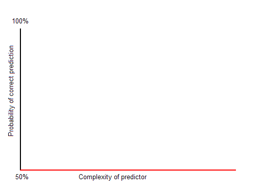
Perfect prediction in the real world can be very, very complex, or even infinitely complex. That means that there isn't enough time or space to do the job perfectly. As someone else has noted (Arthur C. Clark?), some systems are so complex that the only way to "predict" what happens is to watch the system itself. But even very complex systems may be predictable with high probability, as we have seen. What is the relationship between the complexity of our best predictor and the probability of a correct prediction? This will depend on the system we are predicting--there are many possibilities. Below are some graphs to illustrate predictors of a binary sequence. Recall that a constant "predictor" can't do worse that 50%.

The optimistic case is pictured below. This is embodied in the philosophy of progress--as long as we keep working hard, creating more elaborate (and accurate) formulas, the results will come in the form of better and better predictors.

 The worst case is shown below. No matter how hard we try, we can't do better than guessing. This is the case with radioactive decay (as far as anyone knows).
The graph below is more like the actual progress of science as a "punctuated equilibrium." There are increasingly large complexity deserts, where no improvement is seen. Compare the relatively few scientists that led to Newton's revolution or the efforts of Einstein and his collaborators to the massive undertaking that is string theory (and its competition, like loop quantum gravity).
Note that merely increasing the complexity of a predictor is easy. The hard part is figuring out how to increase prediction rates. You can always make a formula or description more complex, but by doing so it doesn't guarantee that the predictors are any better. Generally speaking, there is no computable (that is, systematic or deterministic) method for automatically finding optimal predictors for a given complexity level. You might think that you could just try every single program of a given complexity level and proceed by exhausting the possibilities, but you run into the Halting Problem. There are practical ways to tackle the problem though. This is a topic from the part of computer science called machine learning. A new tool that appeared this year from Cornell University is Eureqa, a program for finding formulas to fit patterns in data sets using an evolutionary approach.

Next time I will apply this idea to testing and outcomes assessment. It's very cool.

Wednesday, September 02, 2009

Selling Error

In the last few posts I've had fun with the idea that error can have economic value, and that people make money selling it. We probably all do it: we try to edge the odds in our favor when buying a used car (observe its defects to try to negotiate the price down), put new paint on the boat before trying to sell it (to get the price up), wear nice clothes to an interview, and so on. These actions don't affect reality, just its perception.

My main example was SAT coaching, but that horse has been thumped ad nauseum, so I'll give it a rest. Last night I remembered reading a remarkable passage out of Monkey Business by John Rolfe and Peter Troob, subtitled Swinging Through the Wall Street Jungle. John and Peter were new graduates of a fine business school who found out what it's like to be an investment banker. The book is chock-a-block with examples of estimator influence, starting with the gung-ho partner who comes to recruit them painting a picture of (almost) requited greed, luxury, and sophistication. The reality was different, and there's a particular dynamic that I find instructive. First, let them set the stage. The authors describe the competitive environment of investment banking, where banks try to arrange deals (and play middleman, keeping some of the cash torrent that proceeds):
[T]he advisory side of the business has become much more commoditized [than before]. The banker no longer has the lock on relationships. The banker's information is no longer highly proprietary. Information on companies is now so widespread that there's very little company-specific knowledge that bankers can truly call their own. The banker no longer brings enough unique added value to the table to necessarily merit a CEO's granting him a lifelong mandate to provide paid advice on matters of corporate finance.
This describes a shift from a trust relationship based on inside information to a commodity experience. The facts about a company that may be for sale are transparent, so it's up to the bank to find ways to add value to this for the potential buyer. You would think that in a free market what would result is better analysis as the competing investment banks all sharpened their pens to try to outdo each other, right? Wrong.

The real dynamic, according to the narrative, is driven by the loss of trust. In repeated interactions, you are more likely to reciprocate trust. In the "good old days" when a bank was hired to be a long-term advisor, the banker had a vested interest in the relationship continuing. This is not true if the business is one-off, especially when you consider that the people actually making the deal are mostly concerned with their own bonuses and even with the welfare of their own investment bank (my interpolation). Are you more likely to tip a server at a restaurant you visit frequently or one you'll never see again?

This creates a challenge for the banker. How to make my pitch unique? The actual payoff for the buyer is irrelevant, because once the deal is done I have already pocketed my percentage. I think it's obvious that this creates a demand for error: it's in the banker's best interest if the potential clients overestimate the value of the purchase because that increases the probability of the sale. The authors describe how this works when making the pitch. One of the many details described in the text is how to make a bank appear to be the best one for the job. I give excerpts below.
The Expertise section [of the pitch book provided to potential buyers] gives the bankers a chance to perpetrate one of their favorite deceptions--the spinning of the league tables.

The league tables are lists detailing how many deals, representing what total dollar amount, an investment bank has done in a given category. [...] The problem is that only one investment bank can truly be number one for any given type of deal, so the bankers have to get creative.

When spinning the league tables, a banker will steadily whittle down the universe of "appropriate" deals until [his or her] bank comes out number one. There are a million ways to do this. [...] With enough trips to the plastic surgeon, just about any bowlegged trollop can come out looking like a supermodel.

At the end of the day, when the league tables finally make it into the pitch book, the only evidence of subterfuge will e discreet. The heading of the league table will trumpet "Our bank is the top underwriter of IPO's for companies similar to Acme." The caveat, in the form of a footnote in barely legible type at the bottom of the page, will tell the whole story.*

*For IPOs between $50 and $150 million in the telecommunications sector, and excluding foreign issues, real estate investment trusts, and offerings done concurrently with debt issues.
The game is obviously to disguise the bank's true experience with deals of the sort in question. The economic value is perhaps an increased probability of sale. I wonder how effective this game actually is--it seems awfully transparent. The more general principle is that if there is economic value, and you can't affect the actual situation, then try to affect perception of it.

What does this have to do with outcomes assessment? There is a primary lesson to be drawn, I think: avoid competitive relationships in favor of building trust. This is especially true of the relationship between faculty and administration. For example, if outcomes assessments were to be used for assigning merit bonuses to faculty, it would create a competitive environment for the best ratings, giving economic value to the scores. This creates demand for error, which will surely be produced in buckets. This is an argument against high-stakes testing, but especially where the tests or other assessments are complex and easily manipulated.

What would trust-building look like? The obvious things: listen to the bottom-up conversation. Do the faculty actually believe in the assessments, or are they just playing along? Have you used the power of the accreditation bogeyman to ram through changes that almost guarantee the wholesale production of error? When a professor sits down to write an assessment report, what is his or her primary motivation? That's the key question. It would be interesting to do an anonymous survey...

Thursday, August 27, 2009

Amplification Amplification

There's something seductive about self-reference--a topic delightfully expounded in Douglas Hofstadter's book Metamagical Themas. Self-reference shook the foundations of math with the Russell Paradox and then Gödel's incompleteness weirdness. But that doesn't stop the fun--by no means! The latest, coolest application I've seen is the RepRap, which is a machine that can build other things, including itself. I suppose that if the conditions are right it will create a whole ecology of replicator replicators. That's what we are too, of course, just squishier and less prone to rust.

This gratuitous introduction is by way of explaining the title. I've spent some time thinking about Zog's Lemma about the amplification of error, and wondering if there's actually anything there. I think there may be, even in the cold light of the fluorescent sun. I will therefore try to amplify on my prior post.

The idea is this:
As economic value increases, for weak predictors the error of prediction can increase over time.
I opened up WinEdit to try a mathematical formulation, but I haven't gotten too far with that yet. The formality may get in the way anyway. We're considering the prediction of the value of some future valuation. The examples will make it clear, but think Prediction = Actual + Error. The last term could be negative. Consider a couple of scenarios.
1. Imagine pulling a dollar bill from your wallet or handbag. How much is it worth, in dollars? One, right? Well, if you got a fiver by mistake, it's worth five bucks. You're not likely to be convinced by a huckster that your fiver is only really worth one and fork it over for four quarters.
Here we have a situation where predictive error is very low and economic value is low too. The actual value of the dollar is realized when you buy something with it. Let's suppose that a fast food burger is a dollar. If you get a single, it was a dollar. If you get five, it had Lincoln on it.
2. Now imagine that you can't tell the difference between a one dollar bill or a five, or a twenty, or a hundred... You have to depend on "experts" for this. The problem is real because you don't want to walk to the burger stand with a hundred dollar bill; you're just not that hungry. This is not entirely hypothetical: US currency is all the same size, so if you're blind this is the way it is. Euros come in different sizes.
Now the predictor has dropped because you can't be sure whom to trust. There's a chance someone will lie to you when you show them the bill and try to take advantage of you.

Both of these scenarios are with relatively low stakes. The competition for your one dollar or five is not as great as if it were a million, right? What happens when we now consider situations where the economic value of the prediction is high?
3. Airplanes are pretty well understood--just watch this. Predicting what will happen under lots of conditions is achievable. Still, things go wrong once in a while. I think that we can agree that this is high stakes--no need to put a dollar figure on a successful landing.
In this situation, what has happened is that the error has gotten smaller over time. That is, by assiduously investigating every prediction failure, we learn how to make better predictions. This is just how science works, of course.

Now for the weird part. Try to imagine situations where the economic value of the predictor is high, but the accuracy isn't so great. What happens now?
4. You want to plant your crops as soon as possible for economic reasons. The shaman says that the gods have decreed that the last freeze will come late because of some indiscretion within the tribe.
This is deadly serious--if your crop gets frosted over, you may not last the next winter through. But the predictor isn't a very good one. What are the dynamics? In this case, the hapless farmer doesn't have many options. Without an anachronistic scientific approach, there is no way to reduce the error. But that's not the end of the story.

The Shaman has a vested interest in maintaining credibility, no? If it emerges that he's full of buffalo cakes, the tribe may put him out on his ear. Since P = A + E, and (despite his best efforts) he has no way to influence the actual outcome A, nor can he improve his predictions P, his only margin for improvement is E. But how can that be? True, he (or she) can't actually improve the error, but he can try to make it appear so with mystical mumbo-jumbo of sufficient impressiveness. So his best bet is to create the best fakery he can--double and redouble the pageantry and behavior that's so far out of norm that it MUST be profound. A successful faker can then get by without paying any attention to the real problem of prediction, and can just get better and better at pretending to.

The sticky point of this equation--what we need actual math for--is whether Herr Shaman could completely abandon accuracy. Maybe he has some residual knowledge passed down about the seasons, the moon, etc. Can the error rate actually naturally increase in such a situation? Only if the effort in maintaining the better predictor is not more than compensated by an equal effort spent toward new and improved humbug.

But what if we can affect the error ourselves?

5. Odysseus wants to sneak his men past the furious cyclops Polyphemus, who he has just blinded. He and his followers ride underneath sheep so as to fool the giant as he checks who exits by touch. (Homer I ain't.)
The predictor is the cyclops in this high stakes assessment. Odysseus (not being Circe) can't change the fact that his men are men, so the A is immutable. He can only affect the prediction by increasing the error, which he does in fine style. Notice the contrast between this and the previous example. In the previous one, disguising the size of E was done for economic value. Here, E is actually increased as much as possible for the same reason. Odysseus spends a lot of time increasing E, actually.

In common parlance, this is called cheating or manipulation, and it's common even in low-stakes situations as we all know.
But what about the amplification of error I advertised? Glad you asked.

Just imagine a recursive situation like number five above, where there are repeated rounds. Each time, Odysseus tries to sneak by the mutilated son of Poseidon, and each time the cyclops tries to detect him. There are lots of situations like this: they evolve. In biology it's sometimes called a Red Queen Race, after a bit from Alice in Wonderland about running as fast as you can just to stay in place. So we have a curious effect where the predictor P is precariously balanced against the error E, like a tug of war: not moving much perhaps, but with great forces involved.

But there's no reason to assume the playing field is fair. What if the conditions are better for creating E than for eliminating it? That might be the case for the SAT test. The chart below was clipped and pasted together from one in InsideHigherEd yesterday here. It lists year over year improvements in SAT score averages by income range.


It shows convincingly that more money gets you higher scores. Exactly why that's true is debatable, but remember this is an increase for one year. One hypothesis is that students of wealthier families have more access to test preparation and can pay to take the test more times, and probably have parents who enable all this as well as pay for it. Does all this effort increase the teen's actual ability to succeed in college (let's call it A)? Or is it responding to the economic value of the predictor (the SAT score) by increasing E instead?

If it's the latter case, then we have a pretty snapshot of an imperfect estimator demonstrating prediction error on the increase because of economic forces. This would imply that the psychometricians who create and score the SAT haven't found a way to counter the increased error that's hypothesized. Zog's moment in the sun?